
diff options
| author | krakenrf <78108016+krakenrf@users.noreply.github.com> | 2022-11-09 23:33:00 +0100 |
|---|---|---|
| committer | krakenrf <78108016+krakenrf@users.noreply.github.com> | 2022-11-09 23:33:00 +0100 |
| commit | d51adf10ff29f37ccbd62da6b0e208d4fbddd0c7 (patch) | |
| tree | 13225a937db68911b1814166a1e26fb6d48e3cee | |
| parent | Updated Home (markdown) (diff) | |
| download | krakensdr_docs.wiki-d51adf10ff29f37ccbd62da6b0e208d4fbddd0c7.tar krakensdr_docs.wiki-d51adf10ff29f37ccbd62da6b0e208d4fbddd0c7.tar.gz krakensdr_docs.wiki-d51adf10ff29f37ccbd62da6b0e208d4fbddd0c7.tar.bz2 krakensdr_docs.wiki-d51adf10ff29f37ccbd62da6b0e208d4fbddd0c7.tar.lz krakensdr_docs.wiki-d51adf10ff29f37ccbd62da6b0e208d4fbddd0c7.tar.xz krakensdr_docs.wiki-d51adf10ff29f37ccbd62da6b0e208d4fbddd0c7.tar.zst krakensdr_docs.wiki-d51adf10ff29f37ccbd62da6b0e208d4fbddd0c7.zip | |
| -rw-r--r-- | 08.-Passive-Radar.md | 154 |
1 files changed, 0 insertions, 154 deletions
diff --git a/08.-Passive-Radar.md b/08.-Passive-Radar.md deleted file mode 100644 index 7204b88..0000000 --- a/08.-Passive-Radar.md +++ /dev/null @@ -1,154 +0,0 @@ -# Activating Passive Radar Code -The ready to use Pi 4 image comes with the Passive Radar code preinstalled. But by default the DOA software is the one that will run on boot. To change to the passive radar code, connect a monitor and keyboard (or SSH in), and edit `start.sh` in the home folder. You will need to comment out the DOA code run lines, and uncomment the passive radar lines. - -The passive radar code works on both Kraken and Kerberos devices. Make sure that you set a preconfig file that is prefixed with "pr_" for either device. On the Pi 4 image, a "pr_" fixed preconfig is already set by default. (See further below for an explanation on the different "pr_" preconfig files) - -# Passive Radar -Active radar systems emit a radio pulse towards a target such as an aircraft and wait for the reflection of that pulse to return. In contrast, a passive radar system emits no signals. Instead, it makes use of already existing powerful transmitters, such as broadcast FM, TV and mobile phone towers. - -In a basic two channel passive radar system, you have one ‘reference’ antenna pointing towards an ‘illuminator’, aka a powerful radio transmitter. This reference antenna is used to receive a clean copy of the reference signal. - -The second ‘surveillance’ antenna points towards the targets of interest, such as aircraft, cars or marine vessels. The illuminating signal is reflected off the body of these targets, and the reflections are received by the surveillance antenna. - -The reflections are then processed and correlated against the clean reference signal. The result is a ‘bistatic range-doppler’ display that shows detected targets as dots. The position of the dot on the display measures the bistatic velocity of the object, and the bistatic distance. - -## Passive Radar Geometry -In a passive radar system, the geometry of the receiver, transmitter and targets of interest are very important for optimizing performance. - -The targets and illuminator cannot be both in the same direction. The reason is that we want the reference antenna to receive only the direct reference signal, and most importantly we want the surveillance antenna to only receive the reflected signal. If the surveillance antenna is drowned out by the direct reference signal, it will be difficult to determine the reflections only. - -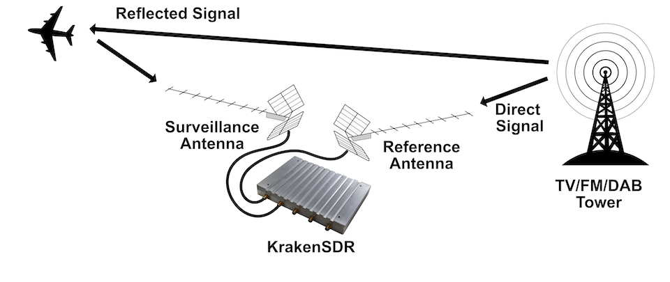 - -## Passive Radar Illuminator Choices -In the modern world there are several possible choices for illuminators. The best characteristics are: - -* **Wideband:** The wider the bandwidth, the greater our radar resolution (up to our maximum 2.56 MHz bandwidth limit) -* **Stable and ‘noise-like’:** HDTV digital signals such as ATSC/DVB-T as well as DAB stations appear noise like in the analogue domain and are desirable. Analogue signals with high variability content like broadcast FM are less desirable. If you must use broadcast FM, a trick is to use heavy metal stations, since heavy metal is closer to white noise. -* **High power:** The higher the transmit power of the illuminating RF source, generally the stronger reflections and more distant reflections will be observed. - -With these characteristics in mind, we recommend using HDTV signals (DVB-T or ATSC), or secondly DAB signals if they exist in your area. Mobile phone 3G/4G/5G signals can also work, but their transmit power is much lower, so they will work only over a smaller area. Broadcast FM is the least desirable due to its small bandwidth and its least noise-like characteristics. - -## Passive Radar Antennas -As per the chapter on passive radar geometry, it is desirable that the reference and surveillance signals are isolated from each other’s antenna. To help with this requirement we can use directional antennas. Directional antennas are antennas that receive with high gain in one direction, and by design attenuate signals in all other directions. - -For basic passive radar you will need two directional antennas, such as Yagi’s. As HDTV signals are perfect for passive radar, it is possible and recommended to use cheap TV Yagi antennas from the local electronics store. - -### Antenna Isolation Tips -As mentioned previously, the reference signal should not be received directly by the surveillance antenna as much as possible. We can achieve that using directional Yagi antennas, but there are some other tricks to improve isolation that can be experimented with. - -The first trick is to use walls, buildings, and other objects to block the reference signal from directly reaching the surveillance antenna. For example, you might have the reference antenna on one side of a building or car, and the surveillance antenna on the other side. - -The second trick is to use polarization to our advantage. A HDTV station may be either horizontally or vertically polarized. The reference Yagi should be oriented with a matching polarization for best reception. However, the surveillance antenna could be oriented in the opposite polarization. The reasoning behind this is that any reflected signals are probably somewhat randomly scattered in terms of polarization, so any antenna orientation should work for the surveillance antenna. And by orienting it in the opposite polarization we get a natural 20dB attenuation of the reference signal. - -# Passive Radar Software -At the time of writing this manual, we have created software that can implement basic 2-channel passive radar. - -Like the direction finding-software, the passive radar software has a configuration and spectrum display screen. The difference is the last page, which is the Passive Radar range-doppler display. - -Note that Receiver 1 is the reference channel. Receiver 2 is the surveillance channel. - -## Passive Radar Configuration Settings - -**Enable Passive Radar:** Enable the passive radar computations to be performed. - -**Clutter Cancellation:** In most scenarios an algorithm to cancel out stationary ‘clutter’ will need to be used, otherwise stationary clutter returns will dominate, hiding the fainter returns from moving objects. At the time of writing this manual there is one clutter cancellation algorithm called “Wiener MRE” implemented. - -**Max Bistatic Range:** How many kilometres of bi-static range to plot on the bi-static range-doppler graph. The choice is dependent on your setup. - -**Max Doppler:** What is the max doppler (speed) reading that should be plotted on the range-doppler graph. - -**PR Persist:** If enabled, the range doppler display will maintain a history of previous plots with some decay value. - -**Persist Decay:** The amount to decay older plot data at each cycle. - -**Dynamic Range:** Choose the plot thresholds for dynamic range. Adjust with trial and error depending on your specific setup until you get a good looking range-doppler graph that shows the moving objects clearly. - -## Passive Radar DAQ Data Block Length / CPI Size Settings Guide -The data block length (aka CPI Size) specifies the length of time radio data is collected. This block of data is then forwarded onwards for DSP processing. - -For passive radar the data block length is an important parameter. Longer data block lengths result in more processing gain (weaker signal detections), and better range-resolution. This comes at the expense of a slower update rate and more CPU processing time. If you run the code on a fast machine, the update rate will be equal to the data block length time. - -Another expense is that fast moving objects could spread their energy out over multiple range-doppler cells if the data block length is too long. - -We have included a preconfigured DAQ file that can be used with an optimized data block length. It is titled `pr_2ch_2pow16`. - -The optimal preconfig file will depend on the specific passive radar implementation and target type. So we recommend experimenting with each of the three preconfig files. - -## Passive Radar Bandwidth Settings Guide -The larger the signal bandwidth the more resolution we can obtain from passive radar. Note that the KrakenSDR is restricted to 125 kHz of bandwidth. - -# Range-Doppler Units -The range-doppler graph displays bistatic range and bistatic speed. The axes are currently described in CELLS. In order to convert cells to meters or m/s use the following formulas: - -$\mathrm{Bistatic Range (meters)} = R_b = cell * \frac{c}{fs}$ - -Where $c$ is the speed of light, and $fs$ is the sample rate (aka bandwidth), and $cell$ is the x-axis cell. The sample rate by default is set to 2.4 MHz. If you have an illumination signal that is smaller, you should set your sample rate to the closest possible bandwidth that matches that illumination signal. - -So for example if we see an object at cell 50 on the x-axis, and we have a sample rate of 2.4 MHz we can calculate $\mathrm{Bistatic Range (meters)} = R_b = 50 * \frac{299792458}{2400000} = 6245 \mathrm{m} = 6.245 \mathrm{km}$ - -For converting doppler cells to Hertz the formula is as follows: - -$\mathrm{Bistatic Frequency (Hz)} = cell * \frac{fs}{2N}$ - -Where $fs$ is the sampling frequency as before, $N$ is the sample size of the coherent processing interval (CPI), and $cell$ is the y-axis cell on the graph. - -In the passive radar software we provide three configuration files `pr_2ch_2pow20`, `pr_2ch_2pow21`, `pr_2ch_2pow22`. In these files the difference is in the CPI value, which is set to $2^{20}$, $2^{21}$ and $2^{22}$ respectively. - -Example cell 500, sampling rate 2.4 MHz and $N = 2^{22}$ - -$\mathrm{Bistatic Frequency (Hz)} = f_b = 500 * \frac{2400000}{2 \times 2^{22}} = 143 \mathrm{Hz}$ - -Then to get to speed in $m.s^{-1}$ we simply multiple the Bistatic Frequency $f_b$ with the wavelength of the illuminator, and multiply by -1. (Positive Doppler decreases the range between you and the target so it has negative speed, it is approaching) - -So if we were using 560 MHz as our illuminator: - -$\mathrm{Bistatic Speed (m.s^{-1})} = -f_b \frac{c}{f} = \frac{299792458}{560000000} \times -143 = 76.5 \mathrm{m.s^{-1}} = 275 \mathrm{km.h^{-1}}$ - -Note that objects moving along the line connecting the transmitter and receiver will always have 0 Hz Doppler shift, as will objects moving around an ellipse of constant bistatic range. - -It is also noted what with increased CPI you receive the benefit of greater bistatic doppler resolution, however range resolution is not increased. Increase CPI does still have the advantages of more processing gain, resulting in weaker reflections being detected. - -# Bistatic Range -The graph provided is a bi-static range doppler graph. Bi-static means that the measurement consists of a transmitter and receiver separated by some distance. This can get complicated, as instead of getting a simple range distance value from the receiver, we end up with an ‘constant range ellipse’ of possible range solutions that depend on some calculations based on the transmitter and receiver positions. - -In the future we aim to have software enhancements that make understanding and visualizing the bistatic range on a map much easier. For now, please keep in mind that the range displayed on the range-doppler graph is not simply just the range from the receiver. - -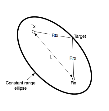 - -The bistatic range displayed on the KrakenSDR range-doppler graph is described by the formula $\mathrm{Bistatic Range (meters)} = R_b = R_{tx} + R_{rx} - L$. So you can see that a single reading on the range-doppler graph describes an ellipse of possible locations. - -For drawing an ellipse we can then use the equation $R_b + L = R_{tx} + R_{rx} = 2a$ - -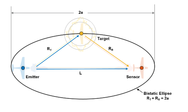 - -(Image Credit: https://www.mathworks.com/help/fusion/ug/track-using-bistatic-range-detections.html) - -You can visualize the value of $R_b + L = R_{tx} + R_{rx} = 2a$ by drawing an ellipse with two pins spaced out at distance $L$, and a piece of string of length $R_b + L$. The ellipse plotted is your contact bistatic range ellipse. The target's position could be anywhere on this ellipse. You can narrow down the possible actual using predefined knowledge of the direction that your surveillance antenna faces, and known knowledge of possible target locations. - -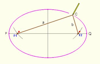 - -(Image Credit: https://www.mathopenref.com/constellipse1.html) - -# Range Resolution -Range resolution depends on the sampling bandwidth, which for the KrakenSDR and RTL-SDR tuners inside is 2.4 MHz. Therefore we achieve $\frac{c}{fs} = \frac{299792458}{2400000} = ~125m$ resolution per range cell on the graph (assuming the illuminating signal is at least 2.4 MHz as well). - -This means that we can differentiate between two different objects that are 125m apart. Or in other words, two objects closer than 125m apart will be combined into a single range cell. - -Another example, if we are using a DAB transmitter as the illuminator, then we only have 1.5 MHz of bandwidth. Therefore we achieve $\frac{c}{fs} = \frac{299792458}{1500000} = ~200m$ resolution per range cell. - -# Other Advanced Passive Radar Notes - -## RD Display within RD Display DVB-T Phenomenon - -Sometimes when using DVB-T as an illuminator you might see shrunken attenuated images of the entire RD display within the RD display itself. This is a phenomenon related to the way in which DVB-T signals are structured for propagation distortion self-correction. It's possible that this could occur with other types of propagation distortion self-correcting signals. - -In brief, the DVB-T signal is constructed in the following way: In the frequency domain we have a vector with 8192 frequency bins. Each of these bins are sub-carriers. Some of these carriers are data carriers, some of them are pilot carriers. The data carriers are used to transfer the useful data (MPEG-2 stream) while the pilot carriers contain fixed modulation data which is preliminary known by the receiver. The transmitter assembles this frequency domain vector (called symbol table) and transforms it to the time domain with iFFT. After transformation it sends out the symbol and assembles the next symbol table. (Of course, there are a lot of other processes besides this main principle but those are not important at the moment). - -The receiver isolates and synchronizes to the symbol in time domain, performs an FFT on the symbol and thus recovers the data carried on the data-carriers. - -Now, as the pilot signals are preliminary known by the receiver it is able to measure what kind of distortion happened with the pilot signals during the propagation and thus determine the response of the radio channel, which is finally used to compensate the data carriers. -From our perspective, the important point is that the pilot carriers are modulated the same way, transfer the same information and they are distributed all across the DVB-T signal spectrum at fixed and scattered positions. - -When we are calculating the range-Doppler map, we are seeking similarities in time-delay and frequency shift (as Doppler). Now, you can imagine that the pilot structure (as mask or frequency domain pattern ) in the received signal matches with its frequency shifted version as the pilots overlap each other. This matching results in dominant correlation peaks in the range-Doppler map. - -A possible solution to clean these out from the range-Doppler map is to construct the so-called missmatched filter. This filter is created by demodulating the received signal, scrambling the pilots and remodulating signal thus constructing a new reference channel.
\ No newline at end of file |